1.9. Tabular Data with Pandas

1.9.1. Introduction

Pandas is a an open source library providing high-performance, easy-to-use data structures and data analysis tools. Pandas is particularly suited to the analysis of tabular data, i.e. data that can can go into a table. In other words, if you can imagine the data in an Excel spreadsheet, then Pandas is the tool for the job.

A 2017 recent analysis of questions from Stack Overflow showed that python was the fastest growing and most widely used programming language in the world (in developed countries). As of 2021, the growth has now leveled off, but Python remains at the top.


Link to generate your own version of this figure

A follow-up analysis showed that this growth is driven by the data science packages such as numpy, matplotlib, and especially pandas.

The exponential growth of pandas is due to the fact that it just works. It saves you time and helps you do science more efficiently and effectively.

Pandas capabilities (from the Pandas website):

• A fast and efficient DataFrame object for data manipulation with integrated indexing;

• Tools for reading and writing data between in-memory data structures and different formats: CSV and text files, Microsoft Excel, SQL databases, and the fast HDF5 format;

• Intelligent data alignment and integrated handling of missing data: gain automatic label-based alignment in computations and easily manipulate messy data into an orderly form;

• Flexible reshaping and pivoting of data sets;

• Intelligent label-based slicing, fancy indexing, and subsetting of large data sets;

• Columns can be inserted and deleted from data structures for size mutability;

• Aggregating or transforming data with a powerful group by engine allowing split-apply-combine operations on data sets;

• High performance merging and joining of data sets;

• Hierarchical axis indexing provides an intuitive way of working with high-dimensional data in a lower-dimensional data structure;

• Time series-functionality: date range generation and frequency conversion, moving window statistics, moving window linear regressions, date shifting and lagging. Even create domain-specific time offsets and join time series without losing data;

• Highly optimized for performance, with critical code paths written in Cython or C.

In this notebook, we will go over the basic capabilities of Pandas. It is a very deep library, and you will need to dig into the documentation for more advanced usage.

Pandas was created by Wes McKinney. Many of the examples here are drawn from Wes McKinney’s book Python for Data Analysis, which includes “a GitHub repo of code samples.

1.9.2. Pandas Data Structures: Series

import pandas as pd
import numpy as np
from matplotlib import pyplot as plt
%matplotlib inline

A Series represents a one-dimensional array of data. The main difference between a Series and numpy array is that a Series has an index. The index contains the labels that we use to access the data.

There are many ways to create a Series. We will just show a few.

(Data are from the NASA Planetary Fact Sheet.)

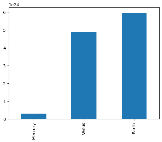
names = ['Mercury', 'Venus', 'Earth']
values = [0.3e24, 4.87e24, 5.97e24]
masses = pd.Series(values, index=names)
masses

Mercury    3.000000e+23
Venus      4.870000e+24
Earth      5.970000e+24
dtype: float64

# Series have built in plotting methods.
masses.plot(kind='bar')

<Axes: >

# Arithmetic operations and most `numpy` function can be applied to Series.
# An important point is that the Series keep their index during such operations.
np.log(masses) / masses**2

Mercury    6.006452e-46
Venus      2.396820e-48
Earth      1.600655e-48
dtype: float64

# We can access the underlying index object if we need to:
masses.index

Index(['Mercury', 'Venus', 'Earth'], dtype='object')

1.9.2.1. Indexing

# We can get values back out using the index via the `.loc` attribute
masses.loc['Earth']

5.97e+24

# Or by raw position using `.iloc`
masses.iloc[2]

5.97e+24

# We can pass a list or array to loc to get multiple rows back:
masses.loc[['Venus', 'Earth']]

Venus    4.870000e+24
Earth    5.970000e+24
dtype: float64

# And we can even use slice notation
masses.loc['Mercury':'Earth']

Mercury    3.000000e+23
Venus      4.870000e+24
Earth      5.970000e+24
dtype: float64

masses.iloc[:2]

Mercury    3.000000e+23
Venus      4.870000e+24
dtype: float64

# If we need to, we can always get the raw data back out as well
masses.values # a numpy array

array([3.00e+23, 4.87e+24, 5.97e+24])

masses.index # a pandas Index object

Index(['Mercury', 'Venus', 'Earth'], dtype='object')

1.9.3. Pandas Data Structures: DataFrame

There is a lot more to Series, but they are limit to a single “column”. A more useful Pandas data structure is the DataFrame. A DataFrame is basically a bunch of series that share the same index. It’s a lot like a table in a spreadsheet.

Below we create a DataFrame.

# first we create a dictionary
data = {'mass': [0.3e24, 4.87e24, 5.97e24],       # kg
        'diameter': [4879e3, 12_104e3, 12_756e3], # m
        'rotation_period': [1407.6, np.nan, 23.9] # h
       }
df = pd.DataFrame(data, index=['Mercury', 'Venus', 'Earth'])
df

	mass	diameter	rotation_period
Mercury	3.000000e+23	4879000.0	1407.6
Venus	4.870000e+24	12104000.0	NaN
Earth	5.970000e+24	12756000.0	23.9

Pandas handles missing data very elegantly, keeping track of it through all calculations.

df.info()

<class 'pandas.core.frame.DataFrame'>
Index: 3 entries, Mercury to Earth
Data columns (total 3 columns):
 #   Column           Non-Null Count  Dtype  
---  ------           --------------  -----  
 0   mass             3 non-null      float64
 1   diameter         3 non-null      float64
 2   rotation_period  2 non-null      float64
dtypes: float64(3)
memory usage: 96.0+ bytes

A wide range of statistical functions are available on both Series and DataFrames.

print(df.min())
print(df.mean())
print(df.std())
print(df.describe())

mass               3.000000e+23
diameter           4.879000e+06
rotation_period    2.390000e+01
dtype: float64
mass               3.713333e+24
diameter           9.913000e+06
rotation_period    7.157500e+02
dtype: float64
mass               3.006765e+24
diameter           4.371744e+06
rotation_period    9.784237e+02
dtype: float64
               mass      diameter  rotation_period
count  3.000000e+00  3.000000e+00         2.000000
mean   3.713333e+24  9.913000e+06       715.750000
std    3.006765e+24  4.371744e+06       978.423653
min    3.000000e+23  4.879000e+06        23.900000
25%    2.585000e+24  8.491500e+06       369.825000
50%    4.870000e+24  1.210400e+07       715.750000
75%    5.420000e+24  1.243000e+07      1061.675000
max    5.970000e+24  1.275600e+07      1407.600000

# We can get a single column as a `Series` using python’s `getitem` syntax on the `DataFrame` object.
print(df['mass'])
# …or using attribute syntax.
print(df.mass)

Mercury    3.000000e+23
Venus      4.870000e+24
Earth      5.970000e+24
Name: mass, dtype: float64
Mercury    3.000000e+23
Venus      4.870000e+24
Earth      5.970000e+24
Name: mass, dtype: float64

# Indexing works very similar to series
print(df.loc['Earth'])
print(df.iloc[2])

mass               5.970000e+24
diameter           1.275600e+07
rotation_period    2.390000e+01
Name: Earth, dtype: float64
mass               5.970000e+24
diameter           1.275600e+07
rotation_period    2.390000e+01
Name: Earth, dtype: float64

# But we can also specify the column we want to access
df.loc['Earth', 'mass']

5.97e+24

df.iloc[0:2, 0]

Mercury    3.000000e+23
Venus      4.870000e+24
Name: mass, dtype: float64

If we make a calculation using columns from the DataFrame, it will keep the same index:

volume =  4/3 * np.pi * (df.diameter/2)**3
df.mass / volume

Mercury    4933.216530
Venus      5244.977070
Earth      5493.285577
dtype: float64

Which we can easily add as another column to the DataFrame:

df['density'] = df.mass / volume
df

	mass	diameter	rotation_period	density
Mercury	3.000000e+23	4879000.0	1407.6	4933.216530
Venus	4.870000e+24	12104000.0	NaN	5244.977070
Earth	5.970000e+24	12756000.0	23.9	5493.285577

1.9.4. Merging Data

Pandas supports a wide range of methods for merging different datasets. These are described extensively in the documentation. Here we just give a few examples.

temperature = pd.Series([167, 464, 15, -65],
                     index=['Mercury', 'Venus', 'Earth', 'Mars'],
                     name='temperature')
temperature

Mercury    167
Venus      464
Earth       15
Mars       -65
Name: temperature, dtype: int64

# returns a new DataFrame
df.join(temperature)

	mass	diameter	rotation_period	density	temperature
Mercury	3.000000e+23	4879000.0	1407.6	4933.216530	167
Venus	4.870000e+24	12104000.0	NaN	5244.977070	464
Earth	5.970000e+24	12756000.0	23.9	5493.285577	15

# returns a new DataFrame
df.join(temperature, how='right')

	mass	diameter	rotation_period	density	temperature
Mercury	3.000000e+23	4879000.0	1407.6	4933.216530	167
Venus	4.870000e+24	12104000.0	NaN	5244.977070	464
Earth	5.970000e+24	12756000.0	23.9	5493.285577	15
Mars	NaN	NaN	NaN	NaN	-65

# returns a new DataFrame
everyone = df.reindex(['Mercury', 'Venus', 'Earth', 'Mars'])
everyone

	mass	diameter	rotation_period	density
Mercury	3.000000e+23	4879000.0	1407.6	4933.216530
Venus	4.870000e+24	12104000.0	NaN	5244.977070
Earth	5.970000e+24	12756000.0	23.9	5493.285577
Mars	NaN	NaN	NaN	NaN

We can also index using a boolean series. This is very useful:

adults = df[df.mass > 4e24]
adults

	mass	diameter	rotation_period	density
Venus	4.870000e+24	12104000.0	NaN	5244.977070
Earth	5.970000e+24	12756000.0	23.9	5493.285577

df['is_big'] = df.mass > 4e24
df

	mass	diameter	rotation_period	density	is_big
Mercury	3.000000e+23	4879000.0	1407.6	4933.216530	False
Venus	4.870000e+24	12104000.0	NaN	5244.977070	True
Earth	5.970000e+24	12756000.0	23.9	5493.285577	True

1.9.5. Modifying Values

We often want to modify values in a dataframe based on some rule. To modify values, we need to use .loc or .iloc

df.loc['Earth', 'mass'] = 5.98+24
df.loc['Venus', 'diameter'] += 1
df

	mass	diameter	rotation_period	density	is_big
Mercury	3.000000e+23	4879000.0	1407.6	4933.216530	False
Venus	4.870000e+24	12104001.0	NaN	5244.977070	True
Earth	2.998000e+01	12756000.0	23.9	5493.285577	True

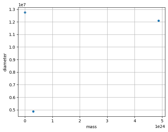
1.9.6. Plotting

DataFrames have all kinds of useful plotting built in.

df.plot(kind='scatter', x='mass', y='diameter', grid=True)

<Axes: xlabel='mass', ylabel='diameter'>

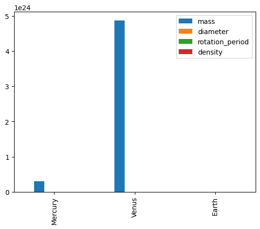
df.plot(kind='bar')

<Axes: >

1.9.7. Time Indexes

Indexes are very powerful. They are a big part of why Pandas is so useful. There are different indexes for different types of data. Time indexes are especially great!

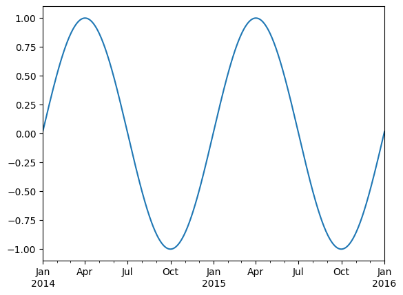
two_years = pd.date_range(start='2014-01-01', end='2016-01-01', freq='D')
timeseries = pd.Series(np.sin(2 *np.pi *two_years.dayofyear / 365),
                       index=two_years)
timeseries.plot()

<Axes: >

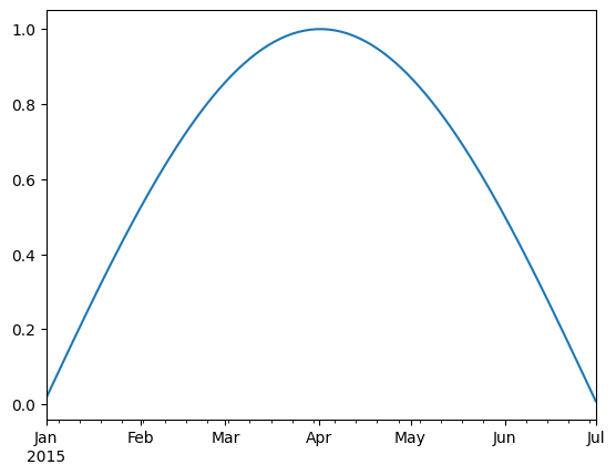
We can use python’s slicing notation inside .loc to select a date range.

timeseries.loc['2015-01-01':'2015-07-01'].plot()

<Axes: >

timeseries.index.month

Index([ 1,  1,  1,  1,  1,  1,  1,  1,  1,  1,
       ...
       12, 12, 12, 12, 12, 12, 12, 12, 12,  1],
      dtype='int32', length=731)

timeseries.index.day

Index([ 1,  2,  3,  4,  5,  6,  7,  8,  9, 10,
       ...
       23, 24, 25, 26, 27, 28, 29, 30, 31,  1],
      dtype='int32', length=731)

1.9.8. Reading Data Files: Weather Station Data

In this example, we will use NOAA weather station data from https://www.ncei.noaa.gov/products/land-based-station.

The details of files we are going to read are described in this README file.

import pooch
POOCH = pooch.create(
    path=pooch.os_cache("noaa-data"),
    base_url="doi:10.5281/zenodo.5564850/",
    registry={
        "data.txt": "md5:5129dcfd19300eb8d4d8d1673fcfbcb4",
    },
)
datafile = POOCH.fetch("data.txt")
datafile

'C:\\Users\\tbeucler\\AppData\\Local\\noaa-data\\noaa-data\\Cache\\data.txt'

! head '/root/.cache/noaa-data/data.txt' # Replace this value with the download path indicated above

'head' is not recognized as an internal or external command,
operable program or batch file.

We now have a text file on our hard drive called data.txt.

To read it into pandas, we will use the read_csv function. This function is incredibly complex and powerful. You can use it to extract data from almost any text file. However, you need to understand how to use its various options.

With no options, this is what we get.

df = pd.read_csv(datafile)
df.head()

	WBANNO LST_DATE CRX_VN LONGITUDE LATITUDE T_DAILY_MAX T_DAILY_MIN T_DAILY_MEAN T_DAILY_AVG P_DAILY_CALC SOLARAD_DAILY SUR_TEMP_DAILY_TYPE SUR_TEMP_DAILY_MAX SUR_TEMP_DAILY_MIN SUR_TEMP_DAILY_AVG RH_DAILY_MAX RH_DAILY_MIN RH_DAILY_AVG SOIL_MOISTURE_5_DAILY SOIL_MOISTURE_10_DAILY SOIL_MOISTURE_20_DAILY SOIL_MOISTURE_50_DAILY SOIL_MOISTURE_100_DAILY SOIL_TEMP_5_DAILY SOIL_TEMP_10_DAILY SOIL_TEMP_20_DAILY SOIL_TEMP_50_DAILY SOIL_TEMP_100_DAILY
0	64756 20170101 2.422 -73.74 41.79 6.6 ...
1	64756 20170102 2.422 -73.74 41.79 4.0 ...
2	64756 20170103 2.422 -73.74 41.79 4.9 ...
3	64756 20170104 2.422 -73.74 41.79 8.7 ...
4	64756 20170105 2.422 -73.74 41.79 -0.5 ...

Pandas failed to identify the different columns. This is because it was expecting standard CSV (comma-separated values) file. In our file, instead, the values are separated by whitespace. And not a single whilespace–the amount of whitespace between values varies. We can tell pandas this using the sep keyword.

df = pd.read_csv(datafile, sep='\s+')
df.head()

	WBANNO	LST_DATE	CRX_VN	LONGITUDE	LATITUDE	T_DAILY_MAX	T_DAILY_MIN	T_DAILY_MEAN	T_DAILY_AVG	P_DAILY_CALC	...	SOIL_MOISTURE_5_DAILY	SOIL_MOISTURE_10_DAILY	SOIL_MOISTURE_20_DAILY	SOIL_MOISTURE_50_DAILY	SOIL_MOISTURE_100_DAILY	SOIL_TEMP_5_DAILY	SOIL_TEMP_10_DAILY	SOIL_TEMP_20_DAILY	SOIL_TEMP_50_DAILY	SOIL_TEMP_100_DAILY
0	64756	20170101	2.422	-73.74	41.79	6.6	-5.4	0.6	2.2	0.0	...	-99.0	-99.0	0.207	0.152	0.175	-0.1	0.0	0.6	1.5	3.4
1	64756	20170102	2.422	-73.74	41.79	4.0	-6.8	-1.4	-1.2	0.0	...	-99.0	-99.0	0.205	0.151	0.173	-0.2	0.0	0.6	1.5	3.3
2	64756	20170103	2.422	-73.74	41.79	4.9	0.7	2.8	2.7	13.1	...	-99.0	-99.0	0.205	0.150	0.173	-0.1	0.0	0.5	1.5	3.3
3	64756	20170104	2.422	-73.74	41.79	8.7	-1.6	3.6	3.5	1.3	...	-99.0	-99.0	0.215	0.153	0.174	-0.1	0.0	0.5	1.5	3.2
4	64756	20170105	2.422	-73.74	41.79	-0.5	-4.6	-2.5	-2.8	0.0	...	-99.0	-99.0	0.215	0.154	0.177	-0.1	0.0	0.5	1.4	3.1

5 rows × 28 columns

Great! It worked.

If we look closely, we will see there are lots of -99 and -9999 values in the file. The README file tells us that these are values used to represent missing data. Let’s tell this to pandas.

df = pd.read_csv(datafile, sep='\s+', na_values=[-9999.0, -99.0])
df.head()

	WBANNO	LST_DATE	CRX_VN	LONGITUDE	LATITUDE	T_DAILY_MAX	T_DAILY_MIN	T_DAILY_MEAN	T_DAILY_AVG	P_DAILY_CALC	...	SOIL_MOISTURE_5_DAILY	SOIL_MOISTURE_10_DAILY	SOIL_MOISTURE_20_DAILY	SOIL_MOISTURE_50_DAILY	SOIL_MOISTURE_100_DAILY	SOIL_TEMP_5_DAILY	SOIL_TEMP_10_DAILY	SOIL_TEMP_20_DAILY	SOIL_TEMP_50_DAILY	SOIL_TEMP_100_DAILY
0	64756	20170101	2.422	-73.74	41.79	6.6	-5.4	0.6	2.2	0.0	...	NaN	NaN	0.207	0.152	0.175	-0.1	0.0	0.6	1.5	3.4
1	64756	20170102	2.422	-73.74	41.79	4.0	-6.8	-1.4	-1.2	0.0	...	NaN	NaN	0.205	0.151	0.173	-0.2	0.0	0.6	1.5	3.3
2	64756	20170103	2.422	-73.74	41.79	4.9	0.7	2.8	2.7	13.1	...	NaN	NaN	0.205	0.150	0.173	-0.1	0.0	0.5	1.5	3.3
3	64756	20170104	2.422	-73.74	41.79	8.7	-1.6	3.6	3.5	1.3	...	NaN	NaN	0.215	0.153	0.174	-0.1	0.0	0.5	1.5	3.2
4	64756	20170105	2.422	-73.74	41.79	-0.5	-4.6	-2.5	-2.8	0.0	...	NaN	NaN	0.215	0.154	0.177	-0.1	0.0	0.5	1.4	3.1

5 rows × 28 columns

Wonderful. The missing data is now represented by NaN.

What data types did pandas infer?

df.info()

<class 'pandas.core.frame.DataFrame'>
RangeIndex: 365 entries, 0 to 364
Data columns (total 28 columns):
 #   Column                   Non-Null Count  Dtype  
---  ------                   --------------  -----  
 0   WBANNO                   365 non-null    int64  
 1   LST_DATE                 365 non-null    int64  
 2   CRX_VN                   365 non-null    float64
 3   LONGITUDE                365 non-null    float64
 4   LATITUDE                 365 non-null    float64
 5   T_DAILY_MAX              364 non-null    float64
 6   T_DAILY_MIN              364 non-null    float64
 7   T_DAILY_MEAN             364 non-null    float64
 8   T_DAILY_AVG              364 non-null    float64
 9   P_DAILY_CALC             364 non-null    float64
 10  SOLARAD_DAILY            364 non-null    float64
 11  SUR_TEMP_DAILY_TYPE      365 non-null    object 
 12  SUR_TEMP_DAILY_MAX       364 non-null    float64
 13  SUR_TEMP_DAILY_MIN       364 non-null    float64
 14  SUR_TEMP_DAILY_AVG       364 non-null    float64
 15  RH_DAILY_MAX             364 non-null    float64
 16  RH_DAILY_MIN             364 non-null    float64
 17  RH_DAILY_AVG             364 non-null    float64
 18  SOIL_MOISTURE_5_DAILY    317 non-null    float64
 19  SOIL_MOISTURE_10_DAILY   317 non-null    float64
 20  SOIL_MOISTURE_20_DAILY   336 non-null    float64
 21  SOIL_MOISTURE_50_DAILY   364 non-null    float64
 22  SOIL_MOISTURE_100_DAILY  359 non-null    float64
 23  SOIL_TEMP_5_DAILY        364 non-null    float64
 24  SOIL_TEMP_10_DAILY       364 non-null    float64
 25  SOIL_TEMP_20_DAILY       364 non-null    float64
 26  SOIL_TEMP_50_DAILY       364 non-null    float64
 27  SOIL_TEMP_100_DAILY      364 non-null    float64
dtypes: float64(25), int64(2), object(1)
memory usage: 80.0+ KB

One problem here is that pandas did not recognize the LST_DATE column as a date. Let’s help it.

df = pd.read_csv(datafile, sep='\s+',
                 na_values=[-9999.0, -99.0],
                 parse_dates=[1])
df.info()

<class 'pandas.core.frame.DataFrame'>
RangeIndex: 365 entries, 0 to 364
Data columns (total 28 columns):
 #   Column                   Non-Null Count  Dtype         
---  ------                   --------------  -----         
 0   WBANNO                   365 non-null    int64         
 1   LST_DATE                 365 non-null    datetime64[ns]
 2   CRX_VN                   365 non-null    float64       
 3   LONGITUDE                365 non-null    float64       
 4   LATITUDE                 365 non-null    float64       
 5   T_DAILY_MAX              364 non-null    float64       
 6   T_DAILY_MIN              364 non-null    float64       
 7   T_DAILY_MEAN             364 non-null    float64       
 8   T_DAILY_AVG              364 non-null    float64       
 9   P_DAILY_CALC             364 non-null    float64       
 10  SOLARAD_DAILY            364 non-null    float64       
 11  SUR_TEMP_DAILY_TYPE      365 non-null    object        
 12  SUR_TEMP_DAILY_MAX       364 non-null    float64       
 13  SUR_TEMP_DAILY_MIN       364 non-null    float64       
 14  SUR_TEMP_DAILY_AVG       364 non-null    float64       
 15  RH_DAILY_MAX             364 non-null    float64       
 16  RH_DAILY_MIN             364 non-null    float64       
 17  RH_DAILY_AVG             364 non-null    float64       
 18  SOIL_MOISTURE_5_DAILY    317 non-null    float64       
 19  SOIL_MOISTURE_10_DAILY   317 non-null    float64       
 20  SOIL_MOISTURE_20_DAILY   336 non-null    float64       
 21  SOIL_MOISTURE_50_DAILY   364 non-null    float64       
 22  SOIL_MOISTURE_100_DAILY  359 non-null    float64       
 23  SOIL_TEMP_5_DAILY        364 non-null    float64       
 24  SOIL_TEMP_10_DAILY       364 non-null    float64       
 25  SOIL_TEMP_20_DAILY       364 non-null    float64       
 26  SOIL_TEMP_50_DAILY       364 non-null    float64       
 27  SOIL_TEMP_100_DAILY      364 non-null    float64       
dtypes: datetime64[ns](1), float64(25), int64(1), object(1)
memory usage: 80.0+ KB

# It worked! Finally, let’s tell pandas to use the date column as the index.
df = df.set_index('LST_DATE')
df.head()

	WBANNO	CRX_VN	LONGITUDE	LATITUDE	T_DAILY_MAX	T_DAILY_MIN	T_DAILY_MEAN	T_DAILY_AVG	P_DAILY_CALC	SOLARAD_DAILY	...	SOIL_MOISTURE_5_DAILY	SOIL_MOISTURE_10_DAILY	SOIL_MOISTURE_20_DAILY	SOIL_MOISTURE_50_DAILY	SOIL_MOISTURE_100_DAILY	SOIL_TEMP_5_DAILY	SOIL_TEMP_10_DAILY	SOIL_TEMP_20_DAILY	SOIL_TEMP_50_DAILY	SOIL_TEMP_100_DAILY
LST_DATE
2017-01-01	64756	2.422	-73.74	41.79	6.6	-5.4	0.6	2.2	0.0	8.68	...	NaN	NaN	0.207	0.152	0.175	-0.1	0.0	0.6	1.5	3.4
2017-01-02	64756	2.422	-73.74	41.79	4.0	-6.8	-1.4	-1.2	0.0	2.08	...	NaN	NaN	0.205	0.151	0.173	-0.2	0.0	0.6	1.5	3.3
2017-01-03	64756	2.422	-73.74	41.79	4.9	0.7	2.8	2.7	13.1	0.68	...	NaN	NaN	0.205	0.150	0.173	-0.1	0.0	0.5	1.5	3.3
2017-01-04	64756	2.422	-73.74	41.79	8.7	-1.6	3.6	3.5	1.3	2.85	...	NaN	NaN	0.215	0.153	0.174	-0.1	0.0	0.5	1.5	3.2
2017-01-05	64756	2.422	-73.74	41.79	-0.5	-4.6	-2.5	-2.8	0.0	4.90	...	NaN	NaN	0.215	0.154	0.177	-0.1	0.0	0.5	1.4	3.1

5 rows × 27 columns

df.loc['2017-08-07']

WBANNO                     64756
CRX_VN                     2.422
LONGITUDE                 -73.74
LATITUDE                   41.79
T_DAILY_MAX                 19.3
T_DAILY_MIN                 12.3
T_DAILY_MEAN                15.8
T_DAILY_AVG                 16.3
P_DAILY_CALC                 4.9
SOLARAD_DAILY               3.93
SUR_TEMP_DAILY_TYPE            C
SUR_TEMP_DAILY_MAX          22.3
SUR_TEMP_DAILY_MIN          11.9
SUR_TEMP_DAILY_AVG          17.7
RH_DAILY_MAX                94.7
RH_DAILY_MIN                76.4
RH_DAILY_AVG                89.5
SOIL_MOISTURE_5_DAILY      0.148
SOIL_MOISTURE_10_DAILY     0.113
SOIL_MOISTURE_20_DAILY     0.094
SOIL_MOISTURE_50_DAILY     0.114
SOIL_MOISTURE_100_DAILY    0.151
SOIL_TEMP_5_DAILY           21.4
SOIL_TEMP_10_DAILY          21.7
SOIL_TEMP_20_DAILY          22.1
SOIL_TEMP_50_DAILY          22.2
SOIL_TEMP_100_DAILY         21.5
Name: 2017-08-07 00:00:00, dtype: object

df.loc['2017-07-01':'2017-07-11']

	WBANNO	CRX_VN	LONGITUDE	LATITUDE	T_DAILY_MAX	T_DAILY_MIN	T_DAILY_MEAN	T_DAILY_AVG	P_DAILY_CALC	SOLARAD_DAILY	...	SOIL_MOISTURE_5_DAILY	SOIL_MOISTURE_10_DAILY	SOIL_MOISTURE_20_DAILY	SOIL_MOISTURE_50_DAILY	SOIL_MOISTURE_100_DAILY	SOIL_TEMP_5_DAILY	SOIL_TEMP_10_DAILY	SOIL_TEMP_20_DAILY	SOIL_TEMP_50_DAILY	SOIL_TEMP_100_DAILY
LST_DATE
2017-07-01	64756	2.422	-73.74	41.79	28.0	19.7	23.9	23.8	0.2	19.28	...	0.157	0.136	0.144	0.129	0.163	25.7	25.4	23.7	21.9	19.9
2017-07-02	64756	2.422	-73.74	41.79	29.8	18.4	24.1	23.7	4.0	27.67	...	0.146	0.135	0.143	0.129	0.162	26.8	26.4	24.5	22.3	20.1
2017-07-03	64756	2.422	-73.74	41.79	28.3	15.0	21.7	21.4	0.0	27.08	...	0.141	0.132	0.139	0.128	0.162	26.4	26.3	24.8	22.8	20.3
2017-07-04	64756	2.422	-73.74	41.79	26.8	12.6	19.7	20.0	0.0	29.45	...	0.131	0.126	0.136	0.126	0.161	25.9	25.8	24.6	22.9	20.6
2017-07-05	64756	2.422	-73.74	41.79	28.0	11.9	20.0	20.7	0.0	26.90	...	0.116	0.114	0.131	0.125	0.161	25.3	25.3	24.2	22.8	20.7
2017-07-06	64756	2.422	-73.74	41.79	25.7	14.3	20.0	20.3	0.0	19.03	...	0.105	0.104	0.126	0.124	0.160	24.7	24.7	23.9	22.7	20.9
2017-07-07	64756	2.422	-73.74	41.79	25.8	16.8	21.3	20.0	11.5	13.88	...	0.114	0.100	0.123	0.123	0.160	24.2	24.2	23.4	22.4	20.8
2017-07-08	64756	2.422	-73.74	41.79	29.0	15.3	22.1	21.5	0.0	21.92	...	0.130	0.106	0.122	0.123	0.159	25.5	25.3	23.9	22.4	20.8
2017-07-09	64756	2.422	-73.74	41.79	26.3	10.9	18.6	19.4	0.0	29.72	...	0.119	0.103	0.119	0.121	0.158	24.8	24.8	23.8	22.5	20.8
2017-07-10	64756	2.422	-73.74	41.79	27.6	11.8	19.7	21.3	0.0	23.67	...	0.105	0.096	0.113	0.120	0.158	24.7	24.7	23.6	22.5	20.9
2017-07-11	64756	2.422	-73.74	41.79	27.4	19.2	23.3	22.6	8.5	17.79	...	0.106	0.093	0.110	0.120	0.157	25.6	25.4	24.1	22.6	20.9

11 rows × 27 columns

1.9.9. Quick statistics

df.describe()

	WBANNO	CRX_VN	LONGITUDE	LATITUDE	T_DAILY_MAX	T_DAILY_MIN	T_DAILY_MEAN	T_DAILY_AVG	P_DAILY_CALC	SOLARAD_DAILY	...	SOIL_MOISTURE_5_DAILY	SOIL_MOISTURE_10_DAILY	SOIL_MOISTURE_20_DAILY	SOIL_MOISTURE_50_DAILY	SOIL_MOISTURE_100_DAILY	SOIL_TEMP_5_DAILY	SOIL_TEMP_10_DAILY	SOIL_TEMP_20_DAILY	SOIL_TEMP_50_DAILY	SOIL_TEMP_100_DAILY
count	365.0	365.000000	365.00	3.650000e+02	364.000000	364.000000	364.000000	364.000000	364.000000	364.000000	...	317.000000	317.000000	336.000000	364.000000	359.000000	364.000000	364.000000	364.000000	364.000000	364.000000
mean	64756.0	2.470767	-73.74	4.179000e+01	15.720055	4.037912	9.876374	9.990110	2.797802	13.068187	...	0.189498	0.183991	0.165470	0.140192	0.160630	12.312637	12.320604	12.060165	11.978022	11.915659
std	0.0	0.085997	0.00	7.115181e-15	10.502087	9.460676	9.727451	9.619168	7.238628	7.953074	...	0.052031	0.054113	0.043989	0.020495	0.016011	9.390034	9.338176	8.767752	8.078346	7.187317
min	64756.0	2.422000	-73.74	4.179000e+01	-12.300000	-21.800000	-17.000000	-16.700000	0.000000	0.100000	...	0.075000	0.078000	0.087000	0.101000	0.117000	-0.700000	-0.400000	0.200000	0.900000	1.900000
25%	64756.0	2.422000	-73.74	4.179000e+01	6.900000	-2.775000	2.100000	2.275000	0.000000	6.225000	...	0.152000	0.139000	0.118750	0.118000	0.154000	2.225000	2.000000	2.475000	3.300000	4.100000
50%	64756.0	2.422000	-73.74	4.179000e+01	17.450000	4.350000	10.850000	11.050000	0.000000	12.865000	...	0.192000	0.198000	0.183000	0.147500	0.165000	13.300000	13.350000	13.100000	12.850000	11.600000
75%	64756.0	2.422000	-73.74	4.179000e+01	24.850000	11.900000	18.150000	18.450000	1.400000	19.740000	...	0.234000	0.227000	0.203000	0.157000	0.173000	21.025000	21.125000	20.400000	19.800000	19.325000
max	64756.0	2.622000	-73.74	4.179000e+01	33.400000	20.700000	25.700000	26.700000	65.700000	29.910000	...	0.296000	0.321000	0.235000	0.182000	0.192000	27.600000	27.400000	25.600000	24.100000	22.100000

8 rows × 26 columns

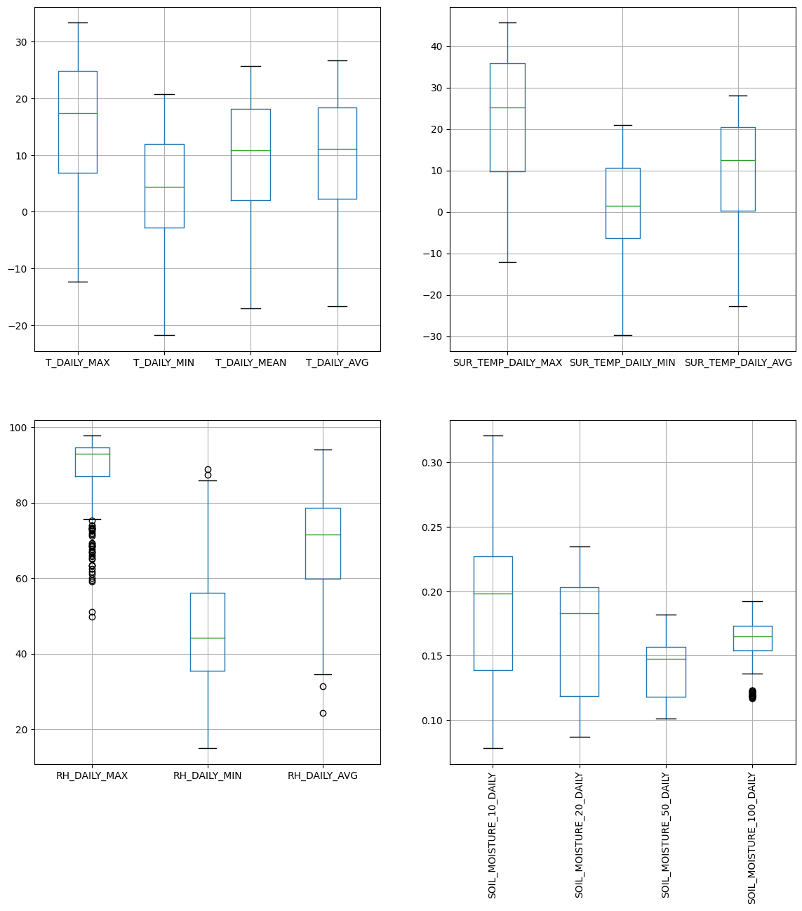
1.9.10. Plotting Values

Pandas integrates a convenient boxplot function:

fig, ax = plt.subplots(ncols=2, nrows=2, figsize=(14,14))

df.iloc[:, 4:8].boxplot(ax=ax[0,0])
df.iloc[:, 10:14].boxplot(ax=ax[0,1])
df.iloc[:, 14:17].boxplot(ax=ax[1,0])
df.iloc[:, 18:22].boxplot(ax=ax[1,1])


ax[1, 1].set_xticklabels(ax[1, 1].get_xticklabels(), rotation=90);

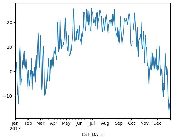
# Pandas is "TIME-AWARE"
df.T_DAILY_MEAN.plot()

<Axes: xlabel='LST_DATE'>

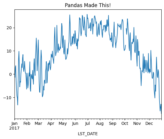
Note: we could also manually create an axis and plot into it.

fig, ax = plt.subplots()
df.T_DAILY_MEAN.plot(ax=ax)
ax.set_title('Pandas Made This!')

Text(0.5, 1.0, 'Pandas Made This!')

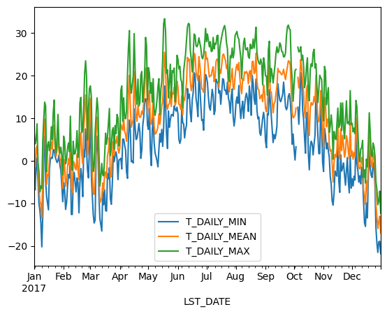
df[['T_DAILY_MIN', 'T_DAILY_MEAN', 'T_DAILY_MAX']].plot()

<Axes: xlabel='LST_DATE'>

1.9.11. Resampling

Since pandas understands time, we can use it to do resampling. The frequency string of each date offset is listed in the time series documentation.

# monthly reampler object
rs_obj = df.resample('MS')
rs_obj

<pandas.core.resample.DatetimeIndexResampler object at 0x00000232EDE79730>

rs_obj.mean()

---------------------------------------------------------------------------
NotImplementedError                       Traceback (most recent call last)
File ~\.conda\envs\JB\lib\site-packages\pandas\core\groupby\groupby.py:1490, in GroupBy._cython_agg_general.<locals>.array_func(values)
   1489 try:
-> 1490     result = self.grouper._cython_operation(
   1491         "aggregate",
   1492         values,
   1493         how,
   1494         axis=data.ndim - 1,
   1495         min_count=min_count,
   1496         **kwargs,
   1497     )
   1498 except NotImplementedError:
   1499     # generally if we have numeric_only=False
   1500     # and non-applicable functions
   1501     # try to python agg
   1502     # TODO: shouldn't min_count matter?

File ~\.conda\envs\JB\lib\site-packages\pandas\core\groupby\ops.py:959, in BaseGrouper._cython_operation(self, kind, values, how, axis, min_count, **kwargs)
    958 ngroups = self.ngroups
--> 959 return cy_op.cython_operation(
    960     values=values,
    961     axis=axis,
    962     min_count=min_count,
    963     comp_ids=ids,
    964     ngroups=ngroups,
    965     **kwargs,
    966 )

File ~\.conda\envs\JB\lib\site-packages\pandas\core\groupby\ops.py:657, in WrappedCythonOp.cython_operation(self, values, axis, min_count, comp_ids, ngroups, **kwargs)
    649     return self._ea_wrap_cython_operation(
    650         values,
    651         min_count=min_count,
   (...)
    654         **kwargs,
    655     )
--> 657 return self._cython_op_ndim_compat(
    658     values,
    659     min_count=min_count,
    660     ngroups=ngroups,
    661     comp_ids=comp_ids,
    662     mask=None,
    663     **kwargs,
    664 )

File ~\.conda\envs\JB\lib\site-packages\pandas\core\groupby\ops.py:497, in WrappedCythonOp._cython_op_ndim_compat(self, values, min_count, ngroups, comp_ids, mask, result_mask, **kwargs)
    495     return res.T
--> 497 return self._call_cython_op(
    498     values,
    499     min_count=min_count,
    500     ngroups=ngroups,
    501     comp_ids=comp_ids,
    502     mask=mask,
    503     result_mask=result_mask,
    504     **kwargs,
    505 )

File ~\.conda\envs\JB\lib\site-packages\pandas\core\groupby\ops.py:541, in WrappedCythonOp._call_cython_op(self, values, min_count, ngroups, comp_ids, mask, result_mask, **kwargs)
    540 out_shape = self._get_output_shape(ngroups, values)
--> 541 func = self._get_cython_function(self.kind, self.how, values.dtype, is_numeric)
    542 values = self._get_cython_vals(values)

File ~\.conda\envs\JB\lib\site-packages\pandas\core\groupby\ops.py:173, in WrappedCythonOp._get_cython_function(cls, kind, how, dtype, is_numeric)
    171 if "object" not in f.__signatures__:
    172     # raise NotImplementedError here rather than TypeError later
--> 173     raise NotImplementedError(
    174         f"function is not implemented for this dtype: "
    175         f"[how->{how},dtype->{dtype_str}]"
    176     )
    177 return f

NotImplementedError: function is not implemented for this dtype: [how->mean,dtype->object]

During handling of the above exception, another exception occurred:

ValueError                                Traceback (most recent call last)
File ~\.conda\envs\JB\lib\site-packages\pandas\core\nanops.py:1692, in _ensure_numeric(x)
   1691 try:
-> 1692     x = float(x)
   1693 except (TypeError, ValueError):
   1694     # e.g. "1+1j" or "foo"

ValueError: could not convert string to float: 'CCCCCCCCCCCCCCCCCCCCCCCCCCCCCCC'

During handling of the above exception, another exception occurred:

ValueError                                Traceback (most recent call last)
File ~\.conda\envs\JB\lib\site-packages\pandas\core\nanops.py:1696, in _ensure_numeric(x)
   1695 try:
-> 1696     x = complex(x)
   1697 except ValueError as err:
   1698     # e.g. "foo"

ValueError: complex() arg is a malformed string

The above exception was the direct cause of the following exception:

TypeError                                 Traceback (most recent call last)
Cell In[51], line 1
----> 1 rs_obj.mean()

File ~\.conda\envs\JB\lib\site-packages\pandas\core\resample.py:979, in Resampler.mean(self, numeric_only, *args, **kwargs)
    977 maybe_warn_args_and_kwargs(type(self), "mean", args, kwargs)
    978 nv.validate_resampler_func("mean", args, kwargs)
--> 979 return self._downsample("mean", numeric_only=numeric_only)

File ~\.conda\envs\JB\lib\site-packages\pandas\core\resample.py:1297, in DatetimeIndexResampler._downsample(self, how, **kwargs)
   1293     return self.asfreq()
   1295 # we are downsampling
   1296 # we want to call the actual grouper method here
-> 1297 result = obj.groupby(self.grouper, axis=self.axis).aggregate(how, **kwargs)
   1299 return self._wrap_result(result)

File ~\.conda\envs\JB\lib\site-packages\pandas\core\groupby\generic.py:1269, in DataFrameGroupBy.aggregate(self, func, engine, engine_kwargs, *args, **kwargs)
   1266 func = maybe_mangle_lambdas(func)
   1268 op = GroupByApply(self, func, args, kwargs)
-> 1269 result = op.agg()
   1270 if not is_dict_like(func) and result is not None:
   1271     return result

File ~\.conda\envs\JB\lib\site-packages\pandas\core\apply.py:160, in Apply.agg(self)
    157 kwargs = self.kwargs
    159 if isinstance(arg, str):
--> 160     return self.apply_str()
    162 if is_dict_like(arg):
    163     return self.agg_dict_like()

File ~\.conda\envs\JB\lib\site-packages\pandas\core\apply.py:496, in Apply.apply_str(self)
    494     if "axis" in arg_names:
    495         self.kwargs["axis"] = self.axis
--> 496 return self._try_aggregate_string_function(obj, f, *self.args, **self.kwargs)

File ~\.conda\envs\JB\lib\site-packages\pandas\core\apply.py:565, in Apply._try_aggregate_string_function(self, obj, arg, *args, **kwargs)
    563 if f is not None:
    564     if callable(f):
--> 565         return f(*args, **kwargs)
    567     # people may try to aggregate on a non-callable attribute
    568     # but don't let them think they can pass args to it
    569     assert len(args) == 0

File ~\.conda\envs\JB\lib\site-packages\pandas\core\groupby\groupby.py:1855, in GroupBy.mean(self, numeric_only, engine, engine_kwargs)
   1853     return self._numba_agg_general(sliding_mean, engine_kwargs)
   1854 else:
-> 1855     result = self._cython_agg_general(
   1856         "mean",
   1857         alt=lambda x: Series(x).mean(numeric_only=numeric_only),
   1858         numeric_only=numeric_only,
   1859     )
   1860     return result.__finalize__(self.obj, method="groupby")

File ~\.conda\envs\JB\lib\site-packages\pandas\core\groupby\groupby.py:1507, in GroupBy._cython_agg_general(self, how, alt, numeric_only, min_count, **kwargs)
   1503         result = self._agg_py_fallback(values, ndim=data.ndim, alt=alt)
   1505     return result
-> 1507 new_mgr = data.grouped_reduce(array_func)
   1508 res = self._wrap_agged_manager(new_mgr)
   1509 out = self._wrap_aggregated_output(res)

File ~\.conda\envs\JB\lib\site-packages\pandas\core\internals\managers.py:1503, in BlockManager.grouped_reduce(self, func)
   1499 if blk.is_object:
   1500     # split on object-dtype blocks bc some columns may raise
   1501     #  while others do not.
   1502     for sb in blk._split():
-> 1503         applied = sb.apply(func)
   1504         result_blocks = extend_blocks(applied, result_blocks)
   1505 else:

File ~\.conda\envs\JB\lib\site-packages\pandas\core\internals\blocks.py:329, in Block.apply(self, func, **kwargs)
    323 @final
    324 def apply(self, func, **kwargs) -> list[Block]:
    325     """
    326     apply the function to my values; return a block if we are not
    327     one
    328     """
--> 329     result = func(self.values, **kwargs)
    331     return self._split_op_result(result)

File ~\.conda\envs\JB\lib\site-packages\pandas\core\groupby\groupby.py:1503, in GroupBy._cython_agg_general.<locals>.array_func(values)
   1490     result = self.grouper._cython_operation(
   1491         "aggregate",
   1492         values,
   (...)
   1496         **kwargs,
   1497     )
   1498 except NotImplementedError:
   1499     # generally if we have numeric_only=False
   1500     # and non-applicable functions
   1501     # try to python agg
   1502     # TODO: shouldn't min_count matter?
-> 1503     result = self._agg_py_fallback(values, ndim=data.ndim, alt=alt)
   1505 return result

File ~\.conda\envs\JB\lib\site-packages\pandas\core\groupby\groupby.py:1457, in GroupBy._agg_py_fallback(self, values, ndim, alt)
   1452     ser = df.iloc[:, 0]
   1454 # We do not get here with UDFs, so we know that our dtype
   1455 #  should always be preserved by the implemented aggregations
   1456 # TODO: Is this exactly right; see WrappedCythonOp get_result_dtype?
-> 1457 res_values = self.grouper.agg_series(ser, alt, preserve_dtype=True)
   1459 if isinstance(values, Categorical):
   1460     # Because we only get here with known dtype-preserving
   1461     #  reductions, we cast back to Categorical.
   1462     # TODO: if we ever get "rank" working, exclude it here.
   1463     res_values = type(values)._from_sequence(res_values, dtype=values.dtype)

File ~\.conda\envs\JB\lib\site-packages\pandas\core\groupby\ops.py:994, in BaseGrouper.agg_series(self, obj, func, preserve_dtype)
    987 if len(obj) > 0 and not isinstance(obj._values, np.ndarray):
    988     # we can preserve a little bit more aggressively with EA dtype
    989     #  because maybe_cast_pointwise_result will do a try/except
    990     #  with _from_sequence.  NB we are assuming here that _from_sequence
    991     #  is sufficiently strict that it casts appropriately.
    992     preserve_dtype = True
--> 994 result = self._aggregate_series_pure_python(obj, func)
    996 npvalues = lib.maybe_convert_objects(result, try_float=False)
    997 if preserve_dtype:

File ~\.conda\envs\JB\lib\site-packages\pandas\core\groupby\ops.py:1015, in BaseGrouper._aggregate_series_pure_python(self, obj, func)
   1012 splitter = self._get_splitter(obj, axis=0)
   1014 for i, group in enumerate(splitter):
-> 1015     res = func(group)
   1016     res = libreduction.extract_result(res)
   1018     if not initialized:
   1019         # We only do this validation on the first iteration

File ~\.conda\envs\JB\lib\site-packages\pandas\core\groupby\groupby.py:1857, in GroupBy.mean.<locals>.<lambda>(x)
   1853     return self._numba_agg_general(sliding_mean, engine_kwargs)
   1854 else:
   1855     result = self._cython_agg_general(
   1856         "mean",
-> 1857         alt=lambda x: Series(x).mean(numeric_only=numeric_only),
   1858         numeric_only=numeric_only,
   1859     )
   1860     return result.__finalize__(self.obj, method="groupby")

File ~\.conda\envs\JB\lib\site-packages\pandas\core\generic.py:11556, in NDFrame._add_numeric_operations.<locals>.mean(self, axis, skipna, numeric_only, **kwargs)
  11539 @doc(
  11540     _num_doc,
  11541     desc="Return the mean of the values over the requested axis.",
   (...)
  11554     **kwargs,
  11555 ):
> 11556     return NDFrame.mean(self, axis, skipna, numeric_only, **kwargs)

File ~\.conda\envs\JB\lib\site-packages\pandas\core\generic.py:11201, in NDFrame.mean(self, axis, skipna, numeric_only, **kwargs)
  11194 def mean(
  11195     self,
  11196     axis: Axis | None = 0,
   (...)
  11199     **kwargs,
  11200 ) -> Series | float:
> 11201     return self._stat_function(
  11202         "mean", nanops.nanmean, axis, skipna, numeric_only, **kwargs
  11203     )

File ~\.conda\envs\JB\lib\site-packages\pandas\core\generic.py:11158, in NDFrame._stat_function(self, name, func, axis, skipna, numeric_only, **kwargs)
  11154     nv.validate_stat_func((), kwargs, fname=name)
  11156 validate_bool_kwarg(skipna, "skipna", none_allowed=False)
> 11158 return self._reduce(
  11159     func, name=name, axis=axis, skipna=skipna, numeric_only=numeric_only
  11160 )

File ~\.conda\envs\JB\lib\site-packages\pandas\core\series.py:4670, in Series._reduce(self, op, name, axis, skipna, numeric_only, filter_type, **kwds)
   4665     raise TypeError(
   4666         f"Series.{name} does not allow {kwd_name}={numeric_only} "
   4667         "with non-numeric dtypes."
   4668     )
   4669 with np.errstate(all="ignore"):
-> 4670     return op(delegate, skipna=skipna, **kwds)

File ~\.conda\envs\JB\lib\site-packages\pandas\core\nanops.py:96, in disallow.__call__.<locals>._f(*args, **kwargs)
     94 try:
     95     with np.errstate(invalid="ignore"):
---> 96         return f(*args, **kwargs)
     97 except ValueError as e:
     98     # we want to transform an object array
     99     # ValueError message to the more typical TypeError
    100     # e.g. this is normally a disallowed function on
    101     # object arrays that contain strings
    102     if is_object_dtype(args[0]):

File ~\.conda\envs\JB\lib\site-packages\pandas\core\nanops.py:158, in bottleneck_switch.__call__.<locals>.f(values, axis, skipna, **kwds)
    156         result = alt(values, axis=axis, skipna=skipna, **kwds)
    157 else:
--> 158     result = alt(values, axis=axis, skipna=skipna, **kwds)
    160 return result

File ~\.conda\envs\JB\lib\site-packages\pandas\core\nanops.py:421, in _datetimelike_compat.<locals>.new_func(values, axis, skipna, mask, **kwargs)
    418 if datetimelike and mask is None:
    419     mask = isna(values)
--> 421 result = func(values, axis=axis, skipna=skipna, mask=mask, **kwargs)
    423 if datetimelike:
    424     result = _wrap_results(result, orig_values.dtype, fill_value=iNaT)

File ~\.conda\envs\JB\lib\site-packages\pandas\core\nanops.py:727, in nanmean(values, axis, skipna, mask)
    724     dtype_count = dtype
    726 count = _get_counts(values.shape, mask, axis, dtype=dtype_count)
--> 727 the_sum = _ensure_numeric(values.sum(axis, dtype=dtype_sum))
    729 if axis is not None and getattr(the_sum, "ndim", False):
    730     count = cast(np.ndarray, count)

File ~\.conda\envs\JB\lib\site-packages\pandas\core\nanops.py:1699, in _ensure_numeric(x)
   1696             x = complex(x)
   1697         except ValueError as err:
   1698             # e.g. "foo"
-> 1699             raise TypeError(f"Could not convert {x} to numeric") from err
   1700 return x

TypeError: Could not convert CCCCCCCCCCCCCCCCCCCCCCCCCCCCCCC to numeric

# We can chain all of that together
df_mm = df.resample('MS').mean()
df_mm[['T_DAILY_MIN', 'T_DAILY_MEAN', 'T_DAILY_MAX']].plot()

And this concludes this notebook’s tutorial 😀

If you would like to learn more about pandas, check out the groupby tutorial from the Earth and Environmental Data Science book, the Github repository of the Python for Data Analysis, or the pandas community tutorials.