1.9. Tabular Data with Pandas

1.9.1. Introduction

Pandas is a an open source library providing high-performance, easy-to-use data structures and data analysis tools. Pandas is particularly suited to the analysis of tabular data, i.e. data that can can go into a table. In other words, if you can imagine the data in an Excel spreadsheet, then Pandas is the tool for the job.

A 2017 recent analysis of questions from Stack Overflow showed that python was the fastest growing and most widely used programming language in the world (in developed countries). As of 2021, the growth has now leveled off, but Python remains at the top.


Link to generate your own version of this figure

A follow-up analysis showed that this growth is driven by the data science packages such as numpy, matplotlib, and especially pandas.

The exponential growth of pandas is due to the fact that it just works. It saves you time and helps you do science more efficiently and effectively.

Pandas capabilities (from the Pandas website):

• A fast and efficient DataFrame object for data manipulation with integrated indexing;

• Tools for reading and writing data between in-memory data structures and different formats: CSV and text files, Microsoft Excel, SQL databases, and the fast HDF5 format;

• Intelligent data alignment and integrated handling of missing data: gain automatic label-based alignment in computations and easily manipulate messy data into an orderly form;

• Flexible reshaping and pivoting of data sets;

• Intelligent label-based slicing, fancy indexing, and subsetting of large data sets;

• Columns can be inserted and deleted from data structures for size mutability;

• Aggregating or transforming data with a powerful group by engine allowing split-apply-combine operations on data sets;

• High performance merging and joining of data sets;

• Hierarchical axis indexing provides an intuitive way of working with high-dimensional data in a lower-dimensional data structure;

• Time series-functionality: date range generation and frequency conversion, moving window statistics, moving window linear regressions, date shifting and lagging. Even create domain-specific time offsets and join time series without losing data;

• Highly optimized for performance, with critical code paths written in Cython or C.

In this notebook, we will go over the basic capabilities of Pandas. It is a very deep library, and you will need to dig into the documentation for more advanced usage.

Pandas was created by Wes McKinney. Many of the examples here are drawn from Wes McKinney’s book Python for Data Analysis, which includes “a GitHub repo of code samples.

1.9.2. Pandas Data Structures: Series

import pandas as pd
import numpy as np
from matplotlib import pyplot as plt
%matplotlib inline

A Series represents a one-dimensional array of data. The main difference between a Series and numpy array is that a Series has an index. The index contains the labels that we use to access the data.

There are many ways to create a Series. We will just show a few.

(Data are from the NASA Planetary Fact Sheet.)

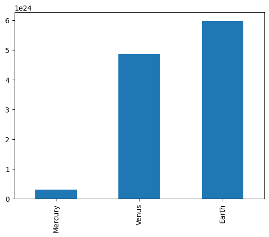
names = ['Mercury', 'Venus', 'Earth']
values = [0.3e24, 4.87e24, 5.97e24]
masses = pd.Series(values, index=names)
masses

Mercury    3.000000e+23
Venus      4.870000e+24
Earth      5.970000e+24
dtype: float64

# Series have built in plotting methods.
masses.plot(kind='bar')

<Axes: >

# Arithmetic operations and most `numpy` function can be applied to Series.
# An important point is that the Series keep their index during such operations.
np.log(masses) / masses**2

Mercury    6.006452e-46
Venus      2.396820e-48
Earth      1.600655e-48
dtype: float64

# We can access the underlying index object if we need to:
masses.index

Index(['Mercury', 'Venus', 'Earth'], dtype='object')

1.9.2.1. Indexing

# We can get values back out using the index via the `.loc` attribute
masses.loc['Earth']

5.97e+24

# Or by raw position using `.iloc`
masses.iloc[2]

5.97e+24

# We can pass a list or array to loc to get multiple rows back:
masses.loc[['Venus', 'Earth']]

Venus    4.870000e+24
Earth    5.970000e+24
dtype: float64

# And we can even use slice notation
masses.loc['Mercury':'Earth']

Mercury    3.000000e+23
Venus      4.870000e+24
Earth      5.970000e+24
dtype: float64

masses.iloc[:2]

Mercury    3.000000e+23
Venus      4.870000e+24
dtype: float64

# If we need to, we can always get the raw data back out as well
masses.values # a numpy array

array([3.00e+23, 4.87e+24, 5.97e+24])

masses.index # a pandas Index object

Index(['Mercury', 'Venus', 'Earth'], dtype='object')

1.9.3. Pandas Data Structures: DataFrame

There is a lot more to Series, but they are limit to a single “column”. A more useful Pandas data structure is the DataFrame. A DataFrame is basically a bunch of series that share the same index. It’s a lot like a table in a spreadsheet.

Below we create a DataFrame.

# first we create a dictionary
data = {'mass': [0.3e24, 4.87e24, 5.97e24],       # kg
        'diameter': [4879e3, 12_104e3, 12_756e3], # m
        'rotation_period': [1407.6, np.nan, 23.9] # h
       }
df = pd.DataFrame(data, index=['Mercury', 'Venus', 'Earth'])
df

	mass	diameter	rotation_period
Mercury	3.000000e+23	4879000.0	1407.6
Venus	4.870000e+24	12104000.0	NaN
Earth	5.970000e+24	12756000.0	23.9

Pandas handles missing data very elegantly, keeping track of it through all calculations.

df.info()

<class 'pandas.core.frame.DataFrame'>
Index: 3 entries, Mercury to Earth
Data columns (total 3 columns):
 #   Column           Non-Null Count  Dtype  
---  ------           --------------  -----  
 0   mass             3 non-null      float64
 1   diameter         3 non-null      float64
 2   rotation_period  2 non-null      float64
dtypes: float64(3)
memory usage: 96.0+ bytes

A wide range of statistical functions are available on both Series and DataFrames.

print(df.min())
print(df.mean())
print(df.std())
print(df.describe())

mass               3.000000e+23
diameter           4.879000e+06
rotation_period    2.390000e+01
dtype: float64
mass               3.713333e+24
diameter           9.913000e+06
rotation_period    7.157500e+02
dtype: float64
mass               3.006765e+24
diameter           4.371744e+06
rotation_period    9.784237e+02
dtype: float64
               mass      diameter  rotation_period
count  3.000000e+00  3.000000e+00         2.000000
mean   3.713333e+24  9.913000e+06       715.750000
std    3.006765e+24  4.371744e+06       978.423653
min    3.000000e+23  4.879000e+06        23.900000
25%    2.585000e+24  8.491500e+06       369.825000
50%    4.870000e+24  1.210400e+07       715.750000
75%    5.420000e+24  1.243000e+07      1061.675000
max    5.970000e+24  1.275600e+07      1407.600000

# We can get a single column as a `Series` using python’s `getitem` syntax on the `DataFrame` object.
print(df['mass'])
# …or using attribute syntax.
print(df.mass)

Mercury    3.000000e+23
Venus      4.870000e+24
Earth      5.970000e+24
Name: mass, dtype: float64
Mercury    3.000000e+23
Venus      4.870000e+24
Earth      5.970000e+24
Name: mass, dtype: float64

# Indexing works very similar to series
print(df.loc['Earth'])
print(df.iloc[2])

mass               5.970000e+24
diameter           1.275600e+07
rotation_period    2.390000e+01
Name: Earth, dtype: float64
mass               5.970000e+24
diameter           1.275600e+07
rotation_period    2.390000e+01
Name: Earth, dtype: float64

# But we can also specify the column we want to access
df.loc['Earth', 'mass']

5.97e+24

df.iloc[0:2, 0]

Mercury    3.000000e+23
Venus      4.870000e+24
Name: mass, dtype: float64

If we make a calculation using columns from the DataFrame, it will keep the same index:

volume =  4/3 * np.pi * (df.diameter/2)**3
df.mass / volume

Mercury    4933.216530
Venus      5244.977070
Earth      5493.285577
dtype: float64

Which we can easily add as another column to the DataFrame:

df['density'] = df.mass / volume
df

	mass	diameter	rotation_period	density
Mercury	3.000000e+23	4879000.0	1407.6	4933.216530
Venus	4.870000e+24	12104000.0	NaN	5244.977070
Earth	5.970000e+24	12756000.0	23.9	5493.285577

1.9.4. Merging Data

Pandas supports a wide range of methods for merging different datasets. These are described extensively in the documentation. Here we just give a few examples.

temperature = pd.Series([167, 464, 15, -65],
                     index=['Mercury', 'Venus', 'Earth', 'Mars'],
                     name='temperature')
temperature

Mercury    167
Venus      464
Earth       15
Mars       -65
Name: temperature, dtype: int64

# returns a new DataFrame
df.join(temperature)

	mass	diameter	rotation_period	density	temperature
Mercury	3.000000e+23	4879000.0	1407.6	4933.216530	167
Venus	4.870000e+24	12104000.0	NaN	5244.977070	464
Earth	5.970000e+24	12756000.0	23.9	5493.285577	15

# returns a new DataFrame
df.join(temperature, how='right')

	mass	diameter	rotation_period	density	temperature
Mercury	3.000000e+23	4879000.0	1407.6	4933.216530	167
Venus	4.870000e+24	12104000.0	NaN	5244.977070	464
Earth	5.970000e+24	12756000.0	23.9	5493.285577	15
Mars	NaN	NaN	NaN	NaN	-65

# returns a new DataFrame
everyone = df.reindex(['Mercury', 'Venus', 'Earth', 'Mars'])
everyone

	mass	diameter	rotation_period	density
Mercury	3.000000e+23	4879000.0	1407.6	4933.216530
Venus	4.870000e+24	12104000.0	NaN	5244.977070
Earth	5.970000e+24	12756000.0	23.9	5493.285577
Mars	NaN	NaN	NaN	NaN

We can also index using a boolean series. This is very useful:

adults = df[df.mass > 4e24]
adults

	mass	diameter	rotation_period	density
Venus	4.870000e+24	12104000.0	NaN	5244.977070
Earth	5.970000e+24	12756000.0	23.9	5493.285577

df['is_big'] = df.mass > 4e24
df

	mass	diameter	rotation_period	density	is_big
Mercury	3.000000e+23	4879000.0	1407.6	4933.216530	False
Venus	4.870000e+24	12104000.0	NaN	5244.977070	True
Earth	5.970000e+24	12756000.0	23.9	5493.285577	True

1.9.5. Modifying Values

We often want to modify values in a dataframe based on some rule. To modify values, we need to use .loc or .iloc

df.loc['Earth', 'mass'] = 5.98+24
df.loc['Venus', 'diameter'] += 1
df

	mass	diameter	rotation_period	density	is_big
Mercury	3.000000e+23	4879000.0	1407.6	4933.216530	False
Venus	4.870000e+24	12104001.0	NaN	5244.977070	True
Earth	2.998000e+01	12756000.0	23.9	5493.285577	True

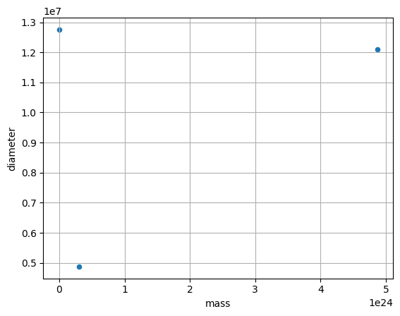
1.9.6. Plotting

DataFrames have all kinds of useful plotting built in.

df.plot(kind='scatter', x='mass', y='diameter', grid=True)

<Axes: xlabel='mass', ylabel='diameter'>

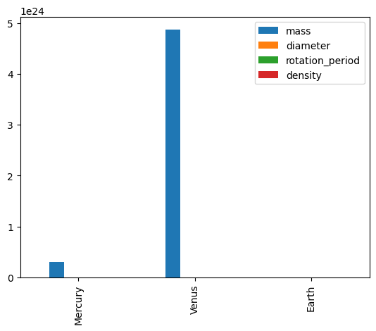
df.plot(kind='bar')

<Axes: >

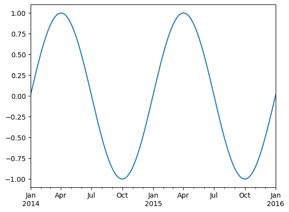
1.9.7. Time Indexes

Indexes are very powerful. They are a big part of why Pandas is so useful. There are different indexes for different types of data. Time indexes are especially great!

two_years = pd.date_range(start='2014-01-01', end='2016-01-01', freq='D')
timeseries = pd.Series(np.sin(2 *np.pi *two_years.dayofyear / 365),
                       index=two_years)
timeseries.plot()

<Axes: >

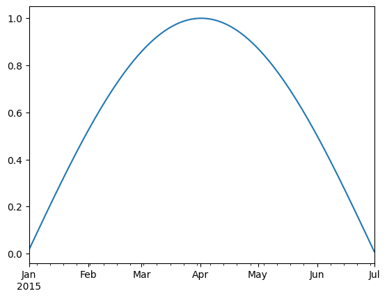
We can use python’s slicing notation inside .loc to select a date range.

timeseries.loc['2015-01-01':'2015-07-01'].plot()

<Axes: >

timeseries.index.month

Index([ 1,  1,  1,  1,  1,  1,  1,  1,  1,  1,
       ...
       12, 12, 12, 12, 12, 12, 12, 12, 12,  1],
      dtype='int32', length=731)

timeseries.index.day

Index([ 1,  2,  3,  4,  5,  6,  7,  8,  9, 10,
       ...
       23, 24, 25, 26, 27, 28, 29, 30, 31,  1],
      dtype='int32', length=731)

1.9.8. Reading Data Files: Weather Station Data

In this example, we will use NOAA weather station data from https://www.ncei.noaa.gov/products/land-based-station.

The details of files we are going to read are described in this README file.

import pooch
POOCH = pooch.create(
    path=pooch.os_cache("noaa-data"),
    base_url="doi:10.5281/zenodo.5564850/",
    registry={
        "data.txt": "md5:5129dcfd19300eb8d4d8d1673fcfbcb4",
    },
)
datafile = POOCH.fetch("data.txt")
datafile

---------------------------------------------------------------------------
ModuleNotFoundError                       Traceback (most recent call last)
Cell In[35], line 1
----> 1 import pooch
      2 POOCH = pooch.create(
      3     path=pooch.os_cache("noaa-data"),
      4     base_url="doi:10.5281/zenodo.5564850/",
   (...)
      7     },
      8 )
      9 datafile = POOCH.fetch("data.txt")

ModuleNotFoundError: No module named 'pooch'

! head '/root/.cache/noaa-data/data.txt' # Replace this value with the download path indicated above

We now have a text file on our hard drive called data.txt.

To read it into pandas, we will use the read_csv function. This function is incredibly complex and powerful. You can use it to extract data from almost any text file. However, you need to understand how to use its various options.

With no options, this is what we get.

df = pd.read_csv(datafile)
df.head()

Pandas failed to identify the different columns. This is because it was expecting standard CSV (comma-separated values) file. In our file, instead, the values are separated by whitespace. And not a single whilespace–the amount of whitespace between values varies. We can tell pandas this using the sep keyword.

df = pd.read_csv(datafile, sep='\s+')
df.head()

Great! It worked.

If we look closely, we will see there are lots of -99 and -9999 values in the file. The README file tells us that these are values used to represent missing data. Let’s tell this to pandas.

df = pd.read_csv(datafile, sep='\s+', na_values=[-9999.0, -99.0])
df.head()

Wonderful. The missing data is now represented by NaN.

What data types did pandas infer?

df.info()

One problem here is that pandas did not recognize the LST_DATE column as a date. Let’s help it.

df = pd.read_csv(datafile, sep='\s+',
                 na_values=[-9999.0, -99.0],
                 parse_dates=[1])
df.info()

# It worked! Finally, let’s tell pandas to use the date column as the index.
df = df.set_index('LST_DATE')
df.head()

df.loc['2017-08-07']

df.loc['2017-07-01':'2017-07-11']

1.9.9. Quick statistics

df.describe()

1.9.10. Plotting Values

Pandas integrates a convenient boxplot function:

fig, ax = plt.subplots(ncols=2, nrows=2, figsize=(14,14))

df.iloc[:, 4:8].boxplot(ax=ax[0,0])
df.iloc[:, 10:14].boxplot(ax=ax[0,1])
df.iloc[:, 14:17].boxplot(ax=ax[1,0])
df.iloc[:, 18:22].boxplot(ax=ax[1,1])


ax[1, 1].set_xticklabels(ax[1, 1].get_xticklabels(), rotation=90);

# Pandas is "TIME-AWARE"
df.T_DAILY_MEAN.plot()

Note: we could also manually create an axis and plot into it.

fig, ax = plt.subplots()
df.T_DAILY_MEAN.plot(ax=ax)
ax.set_title('Pandas Made This!')

df[['T_DAILY_MIN', 'T_DAILY_MEAN', 'T_DAILY_MAX']].plot()

1.9.11. Resampling

Since pandas understands time, we can use it to do resampling. The frequency string of each date offset is listed in the time series documentation.

# monthly reampler object
rs_obj = df.resample('MS')
rs_obj

rs_obj.mean()

# We can chain all of that together
df_mm = df.resample('MS').mean()
df_mm[['T_DAILY_MIN', 'T_DAILY_MEAN', 'T_DAILY_MAX']].plot()

And this concludes this notebook’s tutorial 😀

If you would like to learn more about pandas, check out the groupby tutorial from the Earth and Environmental Data Science book, the Github repository of the Python for Data Analysis, or the pandas community tutorials.