Classification and Regression

2.1. Classification and Regression#

This summary will give you a brief introduction to classification and regression tasks in Machine Learning

Learning Objectives:

Distinguish classification from regression
Define a loss/cost function
Understand how to train a logistic/softmax regression for binary/multiclass classification
Know how to benchmark a classifier

2.1.1. Classification v.s. Regression#

2.1.1.1. Classification#

Classification is a supervised learning task where the model learns to classify instances into predefined classes or categories.

Binary Classification: Classifying instances into two classes (e.g., spam vs. non-spam emails).

Logistic regression is used for binary classification tasks, predicting probabilities for each class.

Log Loss (Cross-Entropy): The cost function used to evaluate the performance of logistic regression models.

Training Logistic Regression: Iteratively optimize the model’s parameters using gradient descent.

Multiclass Classification: Classifying instances into multiple classes (e.g., digit recognition, where each digit is a class).

Multiclass classification, also known as multinomial classification, refers to a classification problem where instances are categorized into three or more distinct classes.

Example: Classifying images of animals into categories like “dog,” “cat,” “elephant,” and “lion.”

Softmax Regression (Multinomial Logistic Regression): Softmax regression is used for multiclass classification tasks, predicting probabilities for multiple classes. The Softmax function ensures the predicted probabilities sum up to 1. Cross-Entropy Loss: The cost function used to evaluate softmax regression models.

Multilabel Classification: Multilabel classification deals with instances that can belong to multiple classes simultaneously. In other words, an instance can have multiple labels associated with it.

Example: Tagging a news article with multiple categories like “politics,” “economy,” and “technology” to capture its diverse content.

Multioutput Classification(or Multioutput Regression):

Multioutput classification (or regression) involves predicting multiple output variables simultaneously for each instance. Each output variable can have multiple possible values or classes.

Example: Predicting both the color and size of a piece of fruit, where color could be “red,” “green,” or “yellow,” and size could be “small,” “medium,” or “large.”

Here are some practical applications of classification in Environmental Sciences🌄

Wildlife Identification: Classification techniques can be used to identify animal species from images or audio recordings, supporting wildlife monitoring projects.

Land Cover Classification: Satellite imagery can be classified into various land cover types, aiding in monitoring land use changes over time.

Invasive Species Detection: Developing models that classify invasive species in images, helping conservationists identify and manage ecological threats.

Water Quality Assessment: Using classification algorithms to determine the quality of water bodies based on factors like chemical concentrations and biological indicators.

2.1.1.2. Regression#

Linear regression is a supervised machine learning algorithm used for predicting a continuous numerical output based on one or more input features. It assumes a linear relationship between the inputs and the target variable. The goal of linear regression is to find the best-fitting line (or hyperplane in higher dimensions) that minimizes the difference between the predicted values and the actual target values. The most common cost function used in linear regression is the Mean Squared Error (MSE).

Multiple linear regression is an extension of linear regression that deals with multiple input features. Instead of just one input, there are multiple independent variables influencing the target variable. The algorithm estimates the coefficients for each feature, determining their individual impact on the target variable while considering their interrelationships.

Other Regression Methods:

Polynomial Regression: This type of regression extends linear regression to capture nonlinear relationships by introducing polynomial terms of the input features. It fits a curve to the data instead of a straight line.

Ridge Regression (L2 Regularization): Ridge regression adds a regularization term to the linear regression cost function. It helps prevent overfitting by penalizing large coefficient values, thus promoting simpler models.

Lasso Regression (L1 Regularization): Similar to ridge regression, lasso regression also adds a regularization term. However, it uses the absolute values of coefficients, often resulting in some coefficients being exactly zero. This leads to feature selection.

Elastic Net Regression: Elastic Net combines L1 and L2 regularization to balance the strengths of both. It can handle situations where there are correlated features.

Support Vector Regression (SVR): SVR applies the principles of support vector machines to regression problems. It aims to fit a hyperplane that captures as many instances within a specified margin as possible.

Decision Tree Regression: Similar to classification decision trees, decision tree regression predicts a continuous target value by partitioning the feature space into regions and assigning the average target value of instances within each region.

Random Forest Regression: An ensemble method combining multiple decision tree regressors. It improves predictive accuracy and reduces overfitting by averaging the predictions of individual trees.

Gradient Boosting Regression: A boosting technique that builds an additive model in a forward stage-wise manner. It combines the predictions of weak learners (often decision trees) to create a strong predictive model.

Each regression method has its own strengths, weaknesses, and applicability to different types of data and problem domains. The choice of which method to use depends on the nature of the data, the problem’s requirements, and the desired level of interpretability and predictive accuracy.

2.1.2. Define Cost Function#

During training, cost Function quantifies the difference betweeen predicted values generated by a model and the actual ground truth values. The cost function is specific to the learning algorithm and is used to update the model’s parameters iteratively to improve its performance on the training data.

The choice of a cost function depends on the nature of the problem—whether it’s a classification, regression, or other type of task—and the desired properties of the model’s predictions. Different algorithms and tasks require different types of cost functions.

Examples:

Mean Squared Error (MSE): Used in regression tasks, it calculates the average squared difference between predicted and actual values. It penalizes larger errors more heavily.

Log Loss (Cross-Entropy Loss): Commonly used in classification tasks, especially in logistic regression and neural networks. It measures the dissimilarity between predicted probabilities and actual binary class labels.

Absolute Error (L1 Loss): Similar to MSE, but it computes the absolute difference between predicted and actual values. It’s less sensitive to outliers compared to MSE.

2.1.3. Training the Model#

2.1.3.1. Gradient Descent#

An optimization technique to minimize the cost function and determine the optimal model parameters. It relies on the partial derivative of the cost function with respect to the model parameters to iteratively improve those parameters. An important parameter of Gradient Descent is the learning rate hyperparameter.

Gradient Descent is an optimization technique used to minimize the cost function and find the optimal model parameters.

Normal Equation vs Gradient Descent

The normal equation provides a closed-form solution to find the optimal parameters that minimize the cost function in linear regression. It is particularly useful when dealing with small to moderately sized datasets as it efficiently computes the optimal parameters directly.

On the other hand, gradient descent is an iterative optimization algorithm that works well with large datasets and complex models. It iteratively updates model parameters in the direction of steepest descent, making it suitable for high-dimensional spaces and non-linear models.

The two methods complement each other in machine learning. While the normal equation offers a straightforward analytical solution for simple cases, gradient descent shines in handling more complex scenarios, where computational efficiency and adaptability to various models and data sizes are paramount.

The optimization techniques using Gradient Descent include the following approaches:

Batch Gradient Descent: Updates model parameters using the entire training set.
Stochastic Gradient Descent (SGD): Updates parameters based on a single training instance or a small batch of instances.
Mini-batch Gradient Descent: A compromise between batch and SGD, updating parameters using a small batch of instances.

Category	Advantages	Disadvantages
Batch Gradient Descent	Stable error gradient	Requires entire training data in memory
	Parallelizable	Slow model updates and convergence
Stochastic Gradient Descent	Avoids stucking in local minimas	Noisy gradient and large variance during training
	Improvements in every model update	Computationally intensive
Mini-batch Gradient Descent	Computationally efficient	Extra hyperparameter to tune
	Smoother learning curves than SGD	Need to accumulate error over batches
	Less memory intensive

2.1.3.2. Learning Rate#

Learning Rate is a small positive scalar value that controls the step size at each iteration during model training. It scales the gradient (derivative) of the loss function with respect to the model parameters.

Impact on Training: A high learning rate can lead to rapid convergence but risks overshooting the optimal solution, potentially causing the model to diverge. Conversely, a low learning rate can lead to slow convergence and might get stuck in local minima.

Learning rate is a crucial hyperparameter in machine learning algorithms, especially those that involve optimization techniques like gradient descent. It determines the size of the steps taken when updating model parameters during the training process. Understanding and setting an appropriate learning rate is vital, as it can significantly impact the training convergence, model performance, and the ability to find the optimal solution. In environmental science, where machine learning is applied to various prediction and forecasting tasks, choosing an appropriate learning rate is essential for achieving accurate and efficient models.

A suitable learning rate is very important and directly affects the likelihood for the ML model to reach the true minima. A small learning rate will result in a slow convergence, whereas a learning rate that is too large might render the model unable to reach the true minima.

Fig 2: An Easy Guide to Gradient Descent in Machine Learning, Great Learning. (link)

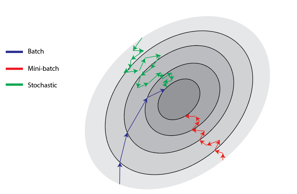
The above figure shows the different ways the three gradient descent methods summarized above approaches the true minima. The SGD can have a very noisy learning process, whereas mini-batch is a compromise between SGD and the smooth batch method.

Fig 3: Relation between Learning Rate and Batch Size, Baeldung. (link)

Some examples:

Air Quality Forecasting: In predicting air quality levels, machine learning models may require careful tuning of the learning rate. An appropriately chosen learning rate can help the model converge to an accurate representation of air quality based on historical data.

Climate Modeling: Climate models often involve complex optimization problems. Setting the learning rate correctly can accelerate the training process and enable better understanding of climate patterns.

Hydrological Forecasting: When predicting river flows or flood levels, an optimal learning rate can ensure that hydrological models converge to accurate predictions, improving early warning systems.

Land Cover Classification: In tasks like land cover classification using remote sensing data, a well-tuned learning rate can help neural networks efficiently learn the intricate relationships between spectral bands and land cover types.

Ecosystem Modeling: Learning rates are essential in ecosystem models, where they affect the speed and stability of parameter estimation, allowing researchers to gain insights into ecosystem dynamics.

2.1.4. Evaluate Model Performance#

In Machine Learning, it is critical to make sure that your trained model can generalize well to unseen data. Model evaluation involves assessing the performance of a trained model using various metrics on a separate dataset (test set or validation set) that the model hasn’t seen during training. For this purpose, we rely on different performance metrics.

The most simple skill score for classification models is the Accuracy Score, which is the ratio between correct predictions and the total number of instances.

The accuracy score is intuitive and straight-forward, but using it to benchmark your classification models can be problematic for real data, particularly if you are dealing with unbalanced data.

Assuming that 90% of your data belongs to the positive class, then the model can have no skills on preddicting negative class and still have a good precision score. 😲 It is definitely not ideal that your classification model can only give you one answer no matter how your samples look like!

Fortunately, we have skill scores that are useful for unbalanced data. These scores balance the precision and the recall of a model.

Precision: The ratio between correctly-predicted positives (True Positive; TP) and the number of instances the model predicted positive (True Positive + False Positive). \ Recall: The ratio between TP and the number of real positives in the data (True Positive + False Negative).

Analyze misclassified instances to gain insights into model weaknesses and potential data issues. We can use a Confusion Matrix table to summary these information in an attractive visual format and how they impact the model’s performance..

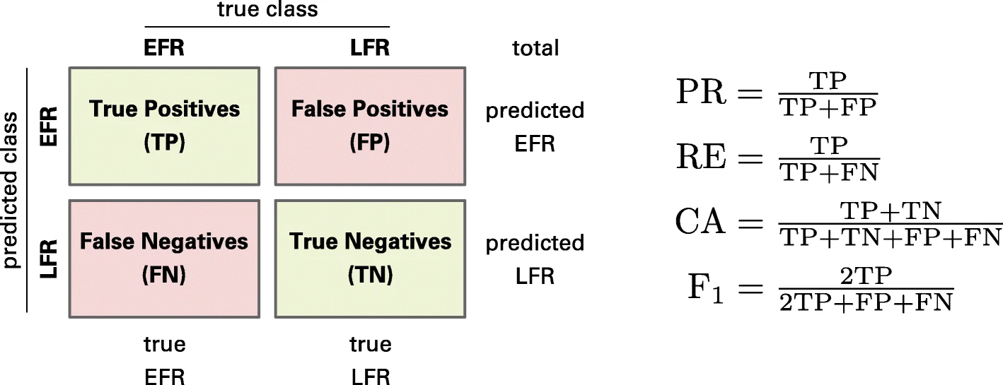
Fig. 1 Confusion matrix (Bittrich et al. 2019)

Scikit-learn provides a function to access the confusion matrix: \ sklearn.metrics.confusion_matrix(y_true, y_pred)

The metric that balances precision and recall is the F1 Score.

F1 Score: The harmonic mean of precision and recall, providing a balanced measure.

ROC-AUC (Receiver Operating Characteristic - Area Under Curve), and PR-AUC (Precision-Recall Area Under Curve) are other metrics used for evaluation.

The ROC curve is a graphical representation that illustrates the trade-off between true positive rate (TPR) and false positive rate (FPR) across various thresholds.

2.1.5. Benchmarking#

Benchmarking a classifier involves assessing its performance against certain metrics and comparing it with other classifiers or established standards.

Tips and Tricks 💡

Overfitting: High-degree polynomials can lead to overfitting the training data.

Learning Rate Scheduling: Adjusting the learning rate during training to converge faster and prevent overshooting.